NetApp

NetApp cDOT – NFS access and export policies

Today I would like to brefily explain terms: export policy and export rule. In Netapp 7-mode if you wanted to create an NFS export you could add an entry to /etc/exports file and export it with exportfs command. In NetApp cDOT it is a different proceedure. To export an share via NFS you have to create an export-policy and assign it to either a Volume or a Qtree that you wish to export.

Another difference is the structure of NFS permissions. in 7-mode if you would like to access via NFS /vol/my_volume/my_qtree, you could just created an exportfs entry for that particular location. In Clustered Data ONTAP NFS clients that have access to the qtree also require at least read-only access at the parent volume and at root level.

You can easily verify that with “export-policy check-access” CLI command, example:

Example 1)

cdot-cluster::> export-policy check-access -vserver svm1 -volume my_volume -qtree my_qtree -access-type read-write -protocol nfs3 -authentication-method sys -client-ip 10.132.0.2
                                         Policy    Policy       Rule
Path                          Policy     Owner     Owner Type  Index Access
----------------------------- ---------- --------- ---------- ------ ----------
/                             root_policy    svm1_root volume 1 read
/vol                          root_policy    svm1_root volume 1 read
/vol/my_volume                     my_volume_policy my_volume volume    2 read
/vol/my_volume/my_qtree              my_qtree_policy my_qtree qtree           1 read-write
4 entries were displayed.

In above example, host 10.132.0.2 has an read-access defined in root_policy and my_volume_policy exports policies. This host has also read-write access defined in rules of my_qtree_policy export policy.

Example 2)

cdot-cluster::> export-policy check-access -vserver svm1 -volume my_volume -qtree my_qtree -access-type read-write -protocol nfs3 -authentication-method sys -client-ip  10.132.0.3
                                         Policy    Policy       Rule
Path                          Policy     Owner     Owner Type  Index Access
----------------------------- ---------- --------- ---------- ------ ----------
/                             root_policy    svm1_root volume 1 read
/vol                          root_policy    svm1_root volume 1 read
/vol/my_volume                       my_volume_policy my_volume volume    0 denied
3 entries were displayed.

In second example host 10.132.0.3 has an read-access defined in root_policy, however it does not have an read-access defined in volume’s policy my_volume_policy. Because of that this host cannot access /vol/my_volume/my_qtree  even if it has read-write access in my_qtree_policy export policy.

Export policy

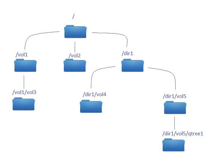
Export policy contain one or more export rule that process each client access request. Each Volume and qtree can have only one export policy assigned, however one export policy might be assigned to many volumes and qtrees. What is important – you cannot assign an export policy to a directory, only to objects like volumes and qtrees. As a consequence you cannot export via NFS a directory  – in opposite to NetApp 7-mode, where it was possible (this article is written when the newest ONTAP version is 9.1).

Export rule

Each rule has an position, and that is the order in which client access is checked.  It means that if you have an export rule (1) saying that 0.0.0.0/0 (all clients) have read-only access, and the rule (2) saying that LinuxRW host has an RW access, LinuxRW in fact will not get  a RW permission, because during client access check, this host was already cought by rule 1, which only gave a RO access. Of course order of rules can be easily modified, it is important to pay attention to it.

NetApp cDOT – Namespace, junction path

One of the biggest difference between “7-mode vs cluster-mode” approach I noticed at the beginning was the term namespace. In 7-mode all volumes were automatically mounted during volume creation to /vol/<vol_name> path. In didn’t matter if the volume was added to vfiler, all volumes on single Data ONTAP 7-mode instance have unique path /vol/<vol_name>. With clustered Data ONTAP the situation is different. Flexible volumes that contain NAS data (basically data served via CIFS or NFS) are junctioned into the owning SVM in a hierarchy.

Junction path

When the flexvol is created, administrator specifies the junction path for that flexible volume. If you have an experience with 7-mode, it’s safe to compare that junction path for 7-mode was set to /vol/<vol_name>. The junction path is a directory location under the root of the SVM where the flexible volume can be accessed.

Namespace and junction paths

Namespace and junction paths

Above you can see an namespace, that have couple of junction paths. / is a root path for SVM (also called SVM root volume). vol1 and vol2 are mounted directly under root path, which means that those can be accessed via SVM1:/vol1 and SVM:/vol2.
vol3 Junction path is /vol1/vol3, which means it can be access via SVM1:/vol1/vol3, also customers who have an access to /vol1, can access vol3 by simply accessing vol3 folder (windows) or directory (unix).
dir1 is a simple directory that doesn’t contain any data, but is used to mount vol4 and vol5 to junction path /dir1/vol4, /dir1/vol5 (if you would like to have same juntion paths as in 7-mode environment you would simply call this directory vol instaed of dir1). Finally there is a qtree created on vol5, since it’s junction path is /dir1/vol5, the path to the qtree is /dir1/vol5/qtree1.

This feature have several advantages. For example NFS clients can access multiple flexible volumes using a single mount point. Same with windows clients, they can access multiple flexvols using a single CIFS share. For example, if your project team need additional capacity for their current action, you can just create a new volume for that, and mount it under the volume that this group have already an access to. In fact – a junction path is independent from a volume name. In other words volume1 can be mounted as /volume1 as well as /current_month.

Namespace example - step 1

Namespace example – step 1

Example:  let’s assume that your customers are storing daily reports to SVM1:/current_month location. At the beginning of march you can create a volume called “march” and junction it to /current_month location. At the end of march you can change this junction to /archive/march, and later on create an “april” volume with junction /current_month.


Namespace example - step 2

Namespace example – step 2

Such operation doesn’t require any action form your customers and doesn’t involve any data movement or data copy on the storage array. It’s a simple modification within your SVM’s namespace.

Namespace

A namespace consists a group of volumes that are connected using junction paths. It’s a hierarchy of all flexible volumes with junction paths within the same SVM (vserver).

Export Policies

I will create a separate entry about this term. Now I would like to briefly introduce it, to explain you another usage of junction paths. An export policy is used to control client access to a specified flexvol. Each flexvol has an export policy associated with it. Multiple volumes can have the same export policy or all of them can have their unique ones. Also qtrees can have theirs unique export policies. Example: you can create a volume “finance” with junction path /finance that can be access only by selected hosts/protocols. In future, when the finance department need a new volume, you can create new_volume with junction path /finance/new_volume. This volume can be accessed only for hosts/protocols that are in-align with “finance” export policy at least on read-level (and additional new_volume policy).

NetApp – Data ONTAP storage architecture – part 1

In my last few posts I started to give you a brief introduction into NetApp clustered Data ONTAP (also called NetApp cDOT or NetApp c-mode). Now, it’s not that easy task, because I don’t know your background. I often assume that you have some general experience working with NetApp 7-mode (“older” mode or concept of managing NetApp storage arrays). But just in case if you don’t in this post I want to go through basic NetApp concepts of storage architecture.

From physical disk to serving data to customers

The architecture of Data ONTAP enables to create logical data volumes that are dynamically mapped to physical space. Let’s take a look at the very beginning.

Physical disks

We have our physical disks – which are packed into disk shelves. Once those disks shelves are connected to Storage Controller(s), the Storage Controller itself must own the disk. Why is that important? In most cases you don’t want to have a single NetApp array, you want to have a cluster of at least 2 nodes to increase the reliability of your storage solution. If you have two nodes (two storage controllers), you want to have an option to fail-over all operations to one controller, if the second one fails, right ? Right – to do so, all physical disks have to be visible by both nodes (both storage controllers). But – during normal operations (both controllers are working as HA – High Availability Pair), you don’t want one controller to “mess with” the others controller data, since those are working independently. That’s why, once you attach physical disks to your cluster and you want to use those disks, you have to decide which controller (node) owns each physical disk.

Disk types

NetApp can work with variety of different disk types. Typically you can devide those disks in terms of use:

  • Capacity – this category describes disks that are lower cost and typically bigger in terms of capacity. Those disks are good to store the data, however they are “slow” in terms of performance. Typically you use those disks if you want to store a copy of your data.  Disks types such as: BSAS, FSAS, mSATA
  • Performance – those are typically SAS or FC-AL disks. However nowadays SAS are the most popular. Those are a little bit more expensive but provides better performance results
  • Ultra-performance – those are solid-sate drives disks, SSD. They are the most expensive in terms of price per 1GB, hoewever they give the best performance results.

RAID groups

OK, we have our disks which are owned by our node (storage controller). It’s a good start, but that’s not everything we need to start serving data to our customers. Next step are RAID groups. Long story short RAID group consists of one or mode disks, and as a group it can either increase the performance (for example RAID-0), or increase the security (for example RAID-1).. Or do both of those (for example RAID-4 or RAID-DP). If you haven’t heard about RAID groups before, that might be a little bit confusing right now. For sake of this article think of RAID group as a bunch of disks that creates a structure on which you put data. This structure can survive a disk failure, and increase performance (comparing to working only on single disks). This definition briefly describes RAID-4. This RAID group is often used in NetApp configurations, however the most popular is RAID-DP. The biggest difference is that RAID-DP can survive two disks failure, and still serve data. How is that possible? Well, it’s possible because those groups are using 1 (for RAID-4) or 2 (for RAID-DP) disks as ‘parity disks’. It means those are not storing customer data itself, but they are used to store “control sum” of those data. In other words if you have 10 disks in RAID-4 configuration it means you have a capacity of 9 disks, since 1 disk is used for parity. If you have 10 disks in RAID-DP confiugration it means you have a capacity of 8 disks, since 2 are used for parity.


That’s the end of part 1. In part 2 I will go futher, explaining how to build aggregates, create volumes and serve files and LUNs to our customers.