Month: September 2016

NetApp cDOT – Drive name formats

In my last two posts I have briefly described Data ONTAP storage architecture (you can find those here: part 1, part 2). In this fairly short entry I want to show you how to identify Your disks within Data ONTAP. Why do you want to do so? Well,  for example – a disk numbering enables you to quickly locate a disk that is associated with a displayed error message.

Data ONTAP 8.2.x and previous

Unfortunately it depends on your Data ONTAP version. With Data ONTAP 8.2.x (and earlier) drive names have different formats, depending on the connection type (FC-AL / SAS). Each drive has a universal unique identifier (UUID) that is a unique number from all other drives in your cluster.

Each disk is named wit their node name at the beginning. For example node1:0b.1.20 (node1 – nodename, 0 – slot, b – port, 1 – shelfID, 20 – bay).

In other words for SAS drives the name convention is <node>:<slot><port>.<shelfID>.<bay>

For SAS in multi-disk shelf the name convention is: <node>:<slot><port>.<shelfID>.<bay>L<position> – <position> is either 1, or 2 – in this shelf type two disks are inside a single bay.

For FC-AL name convention is: <node>:<slot><port>.<loopID>

Node name for unowned disks

As you probably noticed, this naming convention is kind of tricky. In normal HA pair each disks shelf is connected to both nodes. How come can you know which disk is named after which nodename? It’s quite simply actually: if disk is assigned (owned) by this node, it will take its name. If disks is unowned (either broken or unassigned) it will display the alphabetically lowest node name in this HA pair (for example if you have two nodes: cluster1-01, cluster1-02 all your unowned disks will be displayed as cluster1-01:<slot>…

Data ONTAP 8.3.x

Starting from ONTAP 8.3 drive names are independent of what nodes the drive is physically connected to and from which node you can access the drive (Just as a reminder, in healthy cluster drive is physically connected to two nodes  – HA pair, but it’s accessed only by one node – owned by one node).

The drive name name convention is: <stack_id>.<shelf_id>.<bay>.<position>. Let me briefly explain those:

  • stack_id – this value is assgined by Data ONTAP, is unique across the cluster and start with 1.
  • shelf_id – shelf ID is set on the storage shelf when the slehf is added to the stack or loop. Unfortunatelly there is a possibility of shelf ID conflict (two shelves with same shelf_id). In such case shelf_id is replaced with unique shelf serial number.
  • bay – the position of the disk within the shelf.
  • position – used only in multi-disk carrier shelf, when 2 disks can be installed in single bay. This value can be either 1, or 2

Pre-cluster drive name format

Before the node is joined to the cluster it’s disk drive name format is same as it was in Data ONTAP 8.2.x


Shelf id and bay number

You may wonder how to read shelf id and bay number. It depends on the shelf model, however please take a look at this picture:
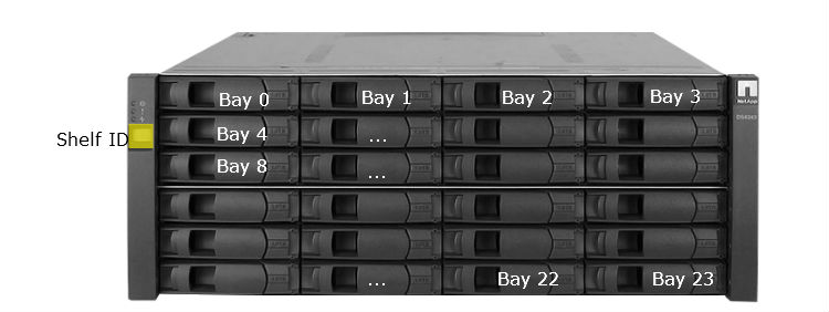
 

DS4243

DS4243

It’s shelf DS4243, that can contain 24 SAS disks (bay numbers from 0 to 23). Shelf ID is a digital number that can be adjusted during shelf installation.

NetApp – Data ONTAP storage architecture – part 2

This is a second part of an introduction to Data ONTAP storage architecture (first part can be found here). In the first part I have briefly describe the two physical layers of a storage architecture: Disks and RAID Groups. There is one more physical layer to introduce – aggregates. Let me start with this one.

Aggregates

Aggregates can be explained as a pool of 4-KB blocks, that gives you the possibility to store data. But to store data you need an physical disks underneath. To gain performance (in terms of I/O) and increase protection NetApp uses RAID groups (RAID-4 or RAID-DP). In other words, Aggregate is nothing more than a bunch of disks. Those disks are combined into one or more RAID group(s). Your NetApp filer can obviously have more than one aggregate. But a single disk can be part of only single raid group and therefore single Aggregate* (* the exeption of that rule would be NetApp Advanced Drive Partitioning, which I will explain in some future entires). But for now, it’s quite safe to remember that single disks can be part only of one aggregate.

Why do you want to have more than one aggregate in your configuration? It’s to support the differing performance, backup, security or data sharing need for your customers. For example one aggregate can be built from ultra-performance SSD disks, where-as second aggregate can be built from capacity – SATA drives.

Aggregate types:

Root / aggr0

This aggregate is atuomatically created during system utilization and it should only contain the node root volume – no user data. Actually within Data ONTAP 8.3.x user data cannot be placed on aggr0 (with older version it is possible, however it’s against the best practices)

Data aggregates

Separate aggregate(s) created especially to serve data to our customers. Those can be single-tiered (built upon same type of disks – for example all HDD or all SSD) or multi-tiered (flash pool) – build with tier of HDDs and SSDs. Currently NetApp enforces a 5-disk minimum to build a data aggregate (3 disks used as “data-disks”, one disk as “parity disk” and one as “dparity disk” in RAID-DP configuration).


FlexVols – Volumes

It’s a first logical layer. A flexvol volume is a volume created on containing aggregate. Single aggregate can have many independent FlexVols. Volumes are managed seperately from the aggregate, you can increase and decrease sizes of a FlexVol without any problems (where-as for aggregates to increase it’s size you have to allocate more physical disks to an aggregate, and you cannot decrease aggregate size). The maximum size of an single volume is 16TB.

Volume is a logical structure that has its own file system.

Thin and thick provisioning

Within FlexVol you have an option to fully guarantee space reservation . What that means is that when you create a 100GB FlexVol, Data ONTAP will reserve 100GB for that FlexVol, and that space will be available only to this volume. This is called thick provisioning. Blocks are not allocated until they are needed, however you guarantee space on the aggregate level the moment you create the volume.

As I mentioned in my previous paragrapth full space guarantee is an option. Within FlexVol you do not have to guarantee space. Volume without that guarantee is thin provisioned. It means the Volume takes only as much space as is actually needed. Back to our previous example, if you create a 100GB thin Volume, it will consume almost nothing on an aggregate at the moment it is created. If you place 20GB data on that Volume, only around 20GB data will be used on aggregate level as well. Why is that cool? Because it gives you the possibility to provision more storage then you currently have, and add additional capacity based on current utilization, not on the requirements. It is much more cost-efficient approach.

Qtrees

Qtree is another logical layer. Qtree enables you to partition the volume into smaller segments which can be managed individually (to some limits). You can for example set the qtree size (by applying quota limit on the qtree), or you can change the security style. You can either export qtree, directory, file or the whole volume to the customers. If you export (via NFS or CIFS) the volume that contains qtrees, customer will see those qtrees as a normal directories (unix) or folders (windows).

LUNs

LUN represents a logical disk that is addressed by a SCSI protocol – it enables block level access. From Data ONTAP point of view single LUN is a single special file that can be accessed via either FC protocol or iSCSI protocol.


Now, please bear in mind – this is just a brief introduction to Data ONTAP storage architecture. In my other posts you can get some additional information.


NetApp – Data ONTAP storage architecture – part 1

In my last few posts I started to give you a brief introduction into NetApp clustered Data ONTAP (also called NetApp cDOT or NetApp c-mode). Now, it’s not that easy task, because I don’t know your background. I often assume that you have some general experience working with NetApp 7-mode (“older” mode or concept of managing NetApp storage arrays). But just in case if you don’t in this post I want to go through basic NetApp concepts of storage architecture.

From physical disk to serving data to customers

The architecture of Data ONTAP enables to create logical data volumes that are dynamically mapped to physical space. Let’s take a look at the very beginning.

Physical disks

We have our physical disks – which are packed into disk shelves. Once those disks shelves are connected to Storage Controller(s), the Storage Controller itself must own the disk. Why is that important? In most cases you don’t want to have a single NetApp array, you want to have a cluster of at least 2 nodes to increase the reliability of your storage solution. If you have two nodes (two storage controllers), you want to have an option to fail-over all operations to one controller, if the second one fails, right ? Right – to do so, all physical disks have to be visible by both nodes (both storage controllers). But – during normal operations (both controllers are working as HA – High Availability Pair), you don’t want one controller to “mess with” the others controller data, since those are working independently. That’s why, once you attach physical disks to your cluster and you want to use those disks, you have to decide which controller (node) owns each physical disk.

Disk types

NetApp can work with variety of different disk types. Typically you can devide those disks in terms of use:

  • Capacity – this category describes disks that are lower cost and typically bigger in terms of capacity. Those disks are good to store the data, however they are “slow” in terms of performance. Typically you use those disks if you want to store a copy of your data.  Disks types such as: BSAS, FSAS, mSATA
  • Performance – those are typically SAS or FC-AL disks. However nowadays SAS are the most popular. Those are a little bit more expensive but provides better performance results
  • Ultra-performance – those are solid-sate drives disks, SSD. They are the most expensive in terms of price per 1GB, hoewever they give the best performance results.

RAID groups

OK, we have our disks which are owned by our node (storage controller). It’s a good start, but that’s not everything we need to start serving data to our customers. Next step are RAID groups. Long story short RAID group consists of one or mode disks, and as a group it can either increase the performance (for example RAID-0), or increase the security (for example RAID-1).. Or do both of those (for example RAID-4 or RAID-DP). If you haven’t heard about RAID groups before, that might be a little bit confusing right now. For sake of this article think of RAID group as a bunch of disks that creates a structure on which you put data. This structure can survive a disk failure, and increase performance (comparing to working only on single disks). This definition briefly describes RAID-4. This RAID group is often used in NetApp configurations, however the most popular is RAID-DP. The biggest difference is that RAID-DP can survive two disks failure, and still serve data. How is that possible? Well, it’s possible because those groups are using 1 (for RAID-4) or 2 (for RAID-DP) disks as ‘parity disks’. It means those are not storing customer data itself, but they are used to store “control sum” of those data. In other words if you have 10 disks in RAID-4 configuration it means you have a capacity of 9 disks, since 1 disk is used for parity. If you have 10 disks in RAID-DP confiugration it means you have a capacity of 8 disks, since 2 are used for parity.


That’s the end of part 1. In part 2 I will go futher, explaining how to build aggregates, create volumes and serve files and LUNs to our customers.